Using CREDO to run and analyse a Suite of Rayleigh-Taylor problems

This examples shows how to use CREDO to run a suite of Underworld runs, based on the same Model XML, but varying different parameters.

Note

This example script is based on the same Rayleigh Taylor model as described in the Using CREDO to run and analyse a Rayleigh-Taylor problem in Underworld section, so please read that section first as it goes into more detail about set-up and results.

Note

This capability of the CREDO toolkit is under active development, so check back here regularly for new features and updates.

Setup

The script to run a suite of Rayleigh Taylor model is as included below, currently in the Underworld/InputFiles directory:

As with the script described in the Basic Ray-Tay example, above the #—————– comment line is setting up and running the model, and that below it is for doing some simple post-processing and analysis of the result.

In this case, as well as setting up a ModelRun object as we did in the basic Ray-Tay example, we also want to create a ModelSuite where the RayTay ModelRun is used as a template (line 11). We then set up the suite to vary the model parameters Gravity, and the amplitude of the Light layer shape (lines 12-17). Finally, on line 18 we request CREDO to run the entire suite. Unlike in the Basic Ray-Tay example, we don’t have to specifically request XMLs records to be saved, the ModelSuite will do this for us automatically.

See also

Modules credo.modelsuite, credo.modelrun, and credo.modelresult.

Looking at the post-processing in more detail:

We are using the Python for control flow statement to loop over each ModelResult in the group of them produced by the ModelSuite [1]. We are also using the saved set of ModelRun objects in the ModelSuite (in the mSuite.runs list) to look up the relevant values for gravity and the shape’s amplitude that were generated from the ranges we specified earlier.

Apart from this, the actual analysis done for each run is the same as in the Basic Ray-Tay example.

See also

The credo.io.stgfreq.FreqOutput class, especially the plotOverTime() method.

Outputs

Since we asked for a suite of ModelRuns, we expect CREDO to run each of the individual runs in turn. The “base” output path requested was output/raytay-suite: this means that CREDO will save the results in here, with individual ModelRuns saved in sub-directories with names based on the parameters involved.

Let’s start with the output produced by running the script at the terminal, which should produce results starting with:

> python credo-rayTaySuite.py 
Running the 12 modelRuns specified in the suite
Doing run 1/12 (index 0), of name 'RayTay-basic':
ModelRun description: "lightLayerAmplitude_0.02-gravity_0.7"
Generating analysis XML:
Running the Model (saving results in output/raytay-suite/lightLayerAmplitude_0.02-gravity_0.7):
Running model 'RayTay-basic' with command 'mpirun -np 1 /home/psunter/AuScopeCodes/stgUnderworldE-credoDev-work/build/bin/StGermain RayleighTaylorBenchmark.xml credo-analysis.xml  --components.lightLayerShape.amplitude=0.02 --gravity=0.7 > logFile.txt' ...
Model ran successfully.
Doing post-run tidyup:

and ending with:

Doing run 12/12 (index 11), of name 'RayTay-basic':
ModelRun description: "lightLayerAmplitude_0.07-gravity_1.0"
Generating analysis XML:
Running the Model (saving results in output/raytay-suite/lightLayerAmplitude_0.07-gravity_1.0):
Running model 'RayTay-basic' with command 'mpirun -np 1 /home/psunter/AuScopeCodes/stgUnderworldE-credoDev-work/build/bin/StGermain RayleighTaylorBenchmark.xml credo-analysis.xml  --components.lightLayerShape.amplitude=0.07 --gravity=1.0 > logFile.txt' ...
Model ran successfully.
Doing post-run tidyup:
Post-process result 0: with gravity=0.7, init perturbation=0.02
	Maximum value of Vrms was 0.000204, at time 62
Post-process result 1: with gravity=0.8, init perturbation=0.02
	Maximum value of Vrms was 0.000262, at time 68
Post-process result 2: with gravity=0.9, init perturbation=0.02
	Maximum value of Vrms was 0.000295, at time 60
Post-process result 3: with gravity=1, init perturbation=0.02
	Maximum value of Vrms was 0.000365, at time 64
Post-process result 4: with gravity=0.7, init perturbation=0.04
	Maximum value of Vrms was 0.000450, at time 66
Post-process result 5: with gravity=0.8, init perturbation=0.04
	Maximum value of Vrms was 0.000548, at time 64
Post-process result 6: with gravity=0.9, init perturbation=0.04
	Maximum value of Vrms was 0.000658, at time 62
Post-process result 7: with gravity=1, init perturbation=0.04
	Maximum value of Vrms was 0.000778, at time 60
Post-process result 8: with gravity=0.7, init perturbation=0.07
	Maximum value of Vrms was 0.000837, at time 63
Post-process result 9: with gravity=0.8, init perturbation=0.07
	Maximum value of Vrms was 0.001038, at time 61
Post-process result 10: with gravity=0.9, init perturbation=0.07
	Maximum value of Vrms was 0.001306, at time 61
Post-process result 11: with gravity=1, init perturbation=0.07
	Maximum value of Vrms was 0.001603, at time 60

You can see the results of our post-processing for loop here, showing how the VRMS value varied in the different runs due to the different input parameters.

Note

In future, this kind of run-comparison capability will be explicitly supported by CREDO, including ability to plot properties of the different runs in the same graph, and save tables of information comparing runs in a text or CSV file.

If you look at the output/raytay-suite directory, you should see a set of sub-directories named:

lightLayerAmplitude_0.02-gravity_0.7
lightLayerAmplitude_0.02-gravity_0.8
lightLayerAmplitude_0.02-gravity_0.9
lightLayerAmplitude_0.02-gravity_1.0
lightLayerAmplitude_0.04-gravity_0.7
lightLayerAmplitude_0.04-gravity_0.8
lightLayerAmplitude_0.04-gravity_0.9
lightLayerAmplitude_0.04-gravity_1.0
lightLayerAmplitude_0.07-gravity_0.7
lightLayerAmplitude_0.07-gravity_0.8
lightLayerAmplitude_0.07-gravity_0.9
lightLayerAmplitude_0.07-gravity_1.0

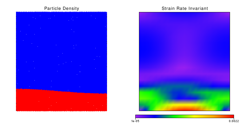
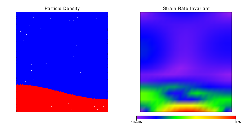
where each of them contains the results of the ModelRun with the parameters set to the given values. The results are as usual for a single ModelRun, as described in the Basic Ray-Tay example. For example, you might like to compare how varying the light layer shape’s amplitude parameter changes the initial conditions of the models by using a file or image browser to examine some of the window.png files. For example, here are two of the images at timestep 1, for a perturbation of 0.02 versus 0.07 respectively:

Each directory will also contain a saved VRMS over time plot, as discussed in Basic Ray-Tay example.

Footnotes

[1]	The ‘enumerate’ is a useful little Python function to also produce an index of each element in a for loop - see its Python documentation.